The gambler's fallacy, a gateway to understanding
What on earth is probability?
Have you ever given any thought to this?
How would you go about explaining probability to an alien with no prior knowledge of human history and culture?
The concept of probability has been approached from many different angles such as subjective and logical standpoints. The epistemology of probability is not my area of expertise but I do like to seize any opportunity I get to point out just how complex things we take for granted really are. Can we objectively and say that probability is the extent to which an event is likely to occur? Or is it something a little more subjective like the strength of our belief that an event is likely to occur? Et cetera.
How we interpret probability changes with time and zeitgeist, the approach most favored these days by scientists and scholars the world over is the frequentist approach (with a respectful nod at the Bayesian approach). At the essence this approach to explain probability is based on an observation most of us have already made. That when similar events are repeated they tend to produce relatively constant frequencies of event outcomes. This is something we are all familiar with, the tendency of a coin to come up heads roughly half of the time or the Red Sox losing 95% of the games I manage to watch is uncanny! The more formal frequentist definition of the probability of an event is the proportion of times that the event would happen in an infinitely long series of repetitions of the scenario. Often referred to as trials. So, to elaborate on the coin toss example above the probability of heads coming up is the proportion of heads against tails in an infinite series of trials. This is hardly achievable in reality as no two trials are exactly the same. The coin wears down with each toss until there’s nothing left along with everything else changing around us constantly. This is of course an ideal and as with other ideas and theories about them we are forced to operationalize and model them in reality, unavoidably introducing errors in our measurements. This is also true of other measurements such as the length of one’s driveway, I can measure it to within one millimeter and get the same results in successive trials but can I measure it to an infinite number of decimal places? I think not.
But I digress. How does all this relate to the title of this post?
The gambler’s fallacy
This notion that random events can follow some kind of pattern even though they are hard to predict demonstrates a huge leap intellectual progress in us humans. While I can’t tell you what number will come up on a d20 (that is a die with twenty sides on it for you not familiar with RPGs such as D&D) I can tell you that in 1000 tosses it will come up around 50 times (although it seldom does when I need it to). Perhaps to underline this leap in understanding of abstract concepts the human brain still struggles with them in everyday circumstances. Even though I’m well aware that every successive throw of the d20 should result in a perfect 20 only 1/20 of the time I’m inclined to believe that if after 2 throws I get 2 perfect 20s I’m due to get something else, perhaps even a couple of 1s!
Enter the gambler’s fallacy.
This idea is nothing new and we still have a hard time getting over it. Even the data seems to support it much of the time with the help of another cognitive bias we so often experience called confirmation bias, also known as cherry picking.
Let’s say I toss a coin ten times and heads come up eight out of those ten times, a proportion of 0.8, some would be inclined to believe that we should have heads come up twice out of the next ten times while in reality heads should come up five times, 8 + 5 = 13 for a proportion of 0.65 out of 20 tosses pulling it closer to the expected 0.5 we should see in infinite tosses (remember the frequentist definition of probability). So instead of saying that the high number of heads early on was countered by an increased number of tails we should rather think of it as diluted as the number of coin tosses increases. This makes sense right?
Ok, let’s add a layer of abstraction to this by introducing a very important concept in probability theory and statistics, two of them actually.
The law of large numbers
What we have just explored regarding the dilution of outcomes with increased number of trials is actually simple way to describe what is known as the law of large numbers, formally defined in the encyclopedia Britannica: > Law of large numbers, in statistics, the theorem that, as the number of identically distributed, > randomly generated variables increases, their sample mean (average) approaches their theoretical > mean. > […] > In coin tossing, the law of large numbers stipulates that the fraction of heads will eventually be > close to 1/2. Hence, if the first 10 tosses produce only 3 heads, it seems that some mystical force > must somehow increase the probability of a head, producing a return of the fraction of heads to its > ultimate limit of 1/2. Yet the law of large numbers requires no such mystical force. Indeed, the > fraction of heads can take a very long time to approach 1/2
But let’s not just take their word for it, let’s try it out!
Consider a set of six values (a six sided die can be used for this experiment):
# create a set of six values from 1 to and including 6
set <- 1:6
# let's view the set
set
## [1] 1 2 3 4 5 6# compute the mean
mean(set)## [1] 3.5So according to the law of large numbers the average of a sample drawn at random with repetition from this number sequence should approach the average of that set. So, the more we throw a six sided die the closer the average of the throws will be to 3.5, the expected value. With repetition basically means you can pick the same number more than once.
Let’s illustrate this:
# set seed for reproducability
set.seed(732928743)

# Let's create a function that simulates throwing a six sided die n number of times
throwDie <- function(n = 30) {

  set <- c(1, 2, 3, 4, 5, 6) # sample space, all the possible sides on the die

  # let's sample a set of n throws based on the number specified
  throws <- sample(set, n, replace=TRUE)

  # We need to aggregate the means from all the throws
  cumulativeSum <- cumsum(throws) # first we use 'cumsum()' to add each throw to the sum of the previous throws
  throwIndex <- c(1:n) # then we need to create an index of the throws
  cumulativeMean <- cumulativeSum / throwIndex # then we compute the mean of each cumulative sum against the index (number of throws)

  return(data.frame(throwIndex, cumulativeMean))
}

# call it
throwDie()
## throwIndex cumulativeMean
## 1 1 6.000000
## 2 2 5.000000
## 3 3 5.333333
## 4 4 5.250000
## 5 5 4.800000
## 6 6 4.333333
## 7 7 4.571429
## 8 8 4.375000
## 9 9 4.000000
## 10 10 3.900000
## 11 11 3.818182
## 12 12 3.666667
## 13 13 3.846154
## 14 14 3.857143
## 15 15 3.866667
## 16 16 3.812500
## 17 17 3.764706
## 18 18 3.611111
## 19 19 3.736842
## 20 20 3.750000
## 21 21 3.714286
## 22 22 3.772727
## 23 23 3.739130
## 24 24 3.666667
## 25 25 3.560000
## 26 26 3.653846
## 27 27 3.629630
## 28 28 3.678571
## 29 29 3.586207
## 30 30 3.566667As you can see from the table above the average approaches the expected value of 3.5 as the number of trials grows. But let’s take this a step further and plot the data so we can get an overview of how the average coincides with the expected value, sometimes it even oscillates around it first!
set.seed(1337)

plotDieThrows <- function(n=800) {
  set <- throwDie(n)
  maxY <- ceiling(max(set$cumulativeMean))
  if(maxY < 5) maxY <- 5
  minY <- floor(min(set$cumulativeMean))
  if(minY > 2) minY <- 2

  finalMean <- round(set$cumulativeMean[n],9)

  # plot the results together
  plot <- plot_ly(set, source = "plot1") %>%
    add_trace(x ~throwIndex, y = ~cumulativeMean,
              type = 'scatter',
              mode = 'lines',
              name = 'Mean',
              text = ~paste0(round(cumulativeMean,2)),
              hoverinfo = 'text') %>%
    add_segments(x = 0,
                 xend = ~ceiling(max(throwIndex)),
                 y = 3.5,
                 yend = 3.5,
                 name = 'Expected value') %>%
    layout(xaxis = list(title = 'Number of throws', tickangle = 45),
           yaxis = list(title = 'Cumulative average',
                        range = c(minY, maxY)),
           annotations = list(
             x = n/2,
             y = maxY - 0.5,
             text = paste("Cumulative mean =",
                          round(finalMean, 2),
                          "\nExpected mean = 3.5",
                          "\nTotal number of throws =",
                          n),
             showarrow = FALSE,
             xanchor = 'left'
           ))

  objList <- list("plot" = plot, "mean" = finalMean)

  return(objList)
}

graphList <- plotDieThrows()

frameWidget(graphList[[1]])
We can see that after 800 throws the mean settles at 3.52, very close to the expected 3.5. You can hover the data points in the plot to see where the mean was at certain points in the process if you want. At the beginning we can see that the average is all over the place but gradually it converges around the expected value. But hang on! Why are we continually adding to the sample by throwing the die again and again? That’s not what you were doing when you threw the d20. You threw it ten times and then ten times again, not 800 times in a row! Correct. And that is also precisely what is done in hypothesis testing which brings us to the other important concept alluded to earlier.
The central limit theorem
The Central Limit Theorem is the limit theorem in probability and statistics. I’m not sure if it’s called the central limit theorem because it’s so important and central to hypothesis testing, but I like to think so.
Instead of sampling values at random from a value set with repetition a set amount of times. I instead repeat the process. So instead of throwing the die 800 times in a row and calculating the average I can draw 80 samples of 10 throws and calculate the average for each sample, giving me a distribution of averages.
Then the Central Limit Theorem states somewhat simplified that if we repeatedly take independent random samples with repetition, the distribution of those sample means will approach a normal distribution (that thing you remember seeing in your intro to stats class), as the number of samples grows.
In other words, if we take simple random samples (with replacement, I really can’t stress this enough) of size 30 from a population and calculate the mean for each of the samples, the distribution of sample means should be approximately normal. You will see the sample size 30 mentioned a lot but the rule is basically this: If you have reason to believe that the underlying population is normally distributed to begin with you can get away with sample sizes of 10 or more, otherwise go with 30 or more.
Let’s visualize this using our trusty (and fair!) six sided die:
set.seed(3426)

throwSampler = function(nObs = 30, nSamples = 500) {

  set <- c(1, 2, 3, 4, 5, 6) # sample space, all the possible sides on the die

  # create a vector to hold the mean from our samples
  sampleDist <- c()

  for (i in 1:nSamples) {
    sampleDist[i] <- mean(sample(set, nObs, replace = TRUE))
  }

  plot <- ggplot() +
            aes(sampleDist) +
            geom_density(aes(y = ..density..)) +
            geom_histogram(aes(y=..density..), alpha = 0.5) +
            geom_vline(xintercept = mean(sampleDist),col="blue",lwd=1.1) +
            ylab("") +
            xlab("Mean") +
            theme(axis.text.y = element_blank())

  return(plot)
}

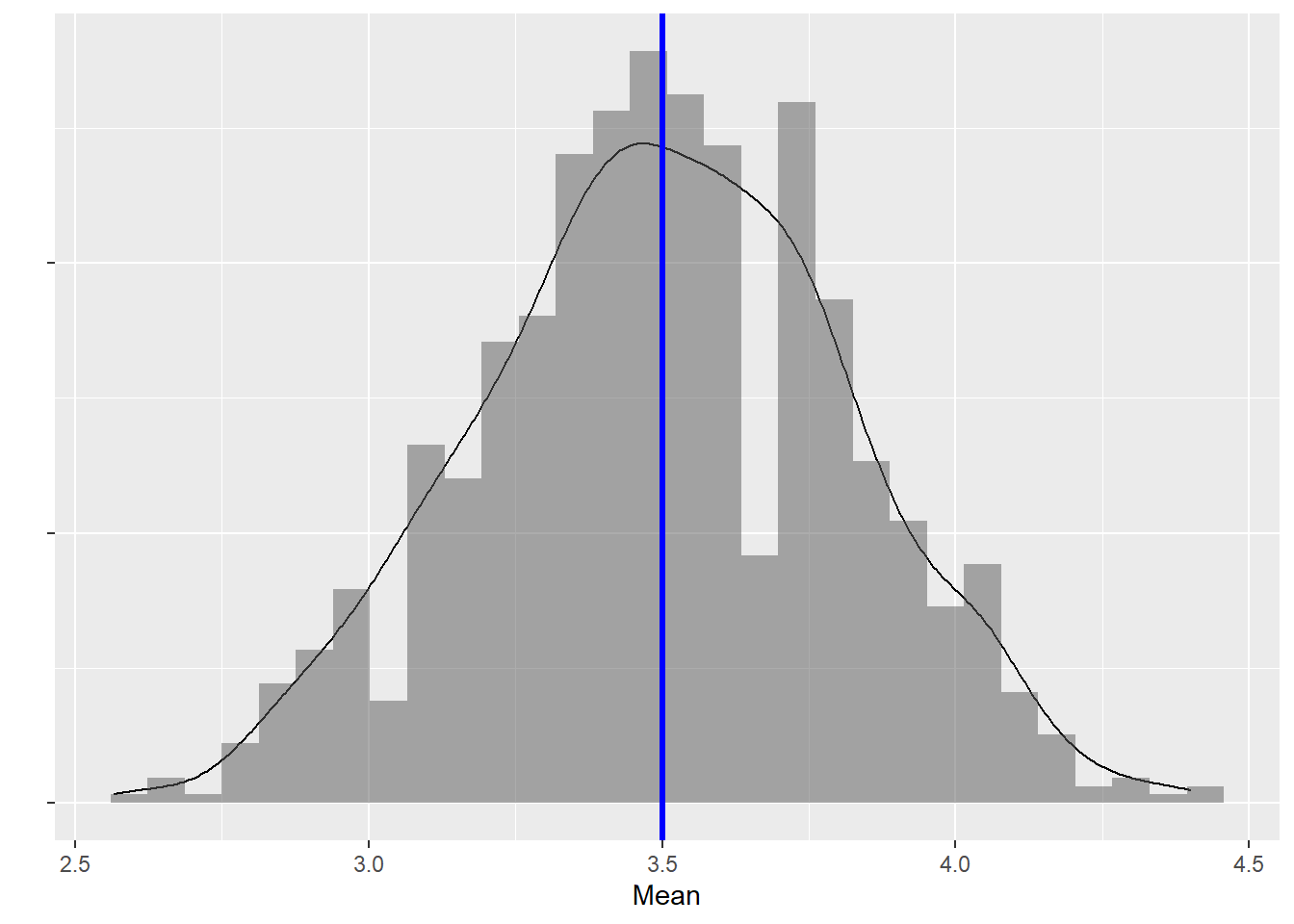
throwSampler(nObs = 30, nSamples = 1000)
So you can see from the above that the main difference between the law of large numbers (LLN) and the Central Limit Theorem (CLT) is that the law of large numbers pertains to one sample while the CLT pertains to the distribution of sample means. What the plot above shows is the mean on the x-axis and the frequency and density probabilities, don’t worry about that for now, what this is supposed to show you is that the sample means are distributed symmetrically around the expected mean of 3.5. But that isn’t really interesting is it? If the die is fair we would expect a sample with mean of 1 in 30 throws to be as likely as a sample with mean of 6. But what if the die isn’t fair?
Let’s do this again, but this time the die isn’t fair.
# set seed for reproducability
set.seed(732928743)

# Let's create a function that simulates throwing a six sided die n number of times
throwDie <- function(n = 30) {

  set <- c(1, 2, 3, 4, 5, 6) # sample space, all the possible sides on the die

  # let's sample a set of n throws based on the number specified
  throws <- sample(set, n, replace=TRUE, prob = c(1, 1, 2, 3, 4, 9)/20) # here we make the die biased

  # We need to aggregate the means from all the throws
  cumulativeSum <- cumsum(throws) # first we use 'cumsum()' to add each throw to the sum of the previous throws
  throwIndex <- c(1:n) # then we need to create an index of the throws
  cumulativeMean <- cumulativeSum / throwIndex # then we compute the mean of each cumulative sum against the index (number of throws)

  return(data.frame(throwIndex, cumulativeMean))
}

# call it
biasedGraph <- plotDieThrows()[[1]]

frameWidget(biasedGraph)
We can see that the die is clearly biased after throwing it 800 times, nothing unexpected happening there.
Now let’s do some sampling.
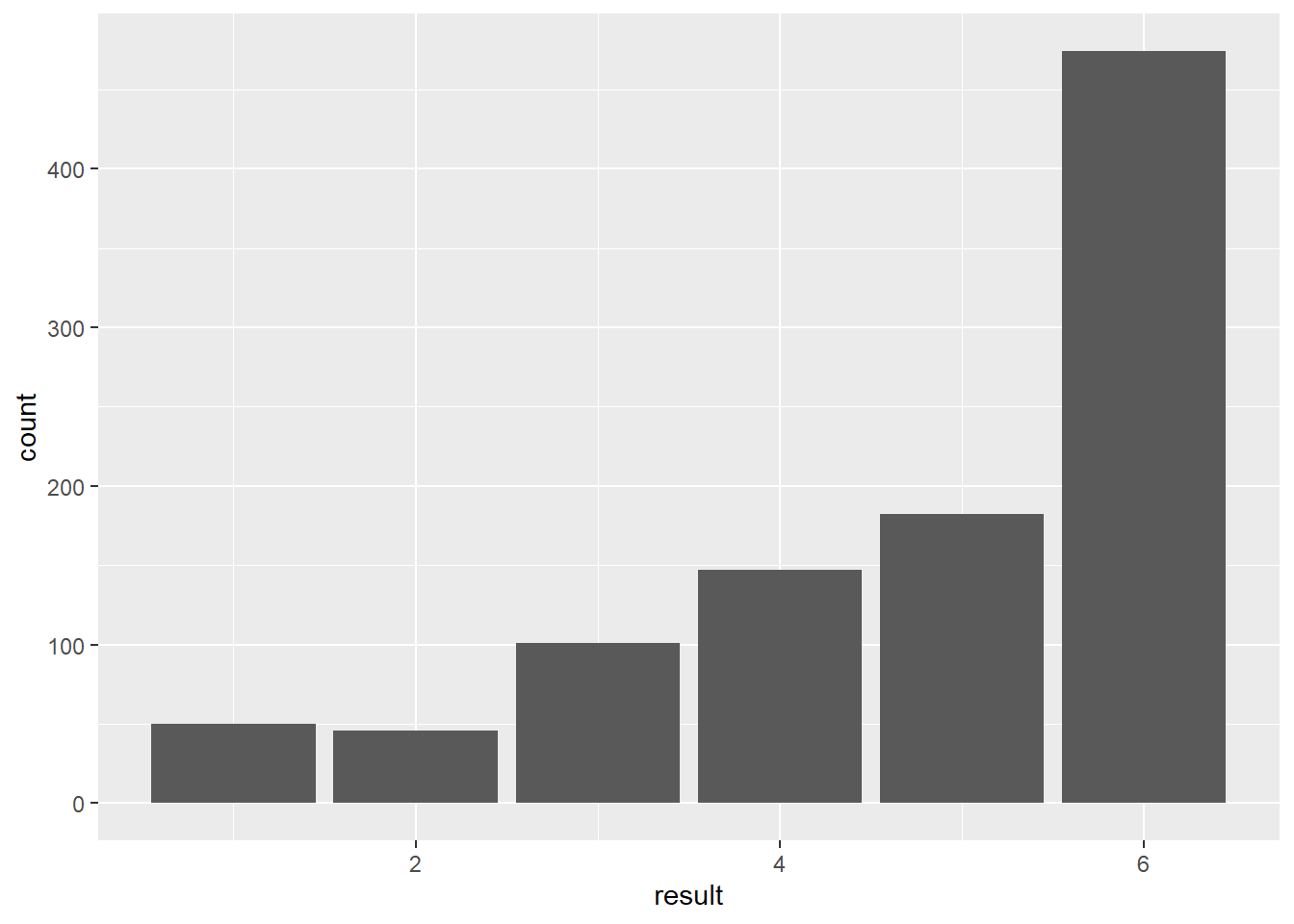
biasedData <- data.frame(index = 1:1000,
                         result = sample(1:6, 1000, replace = TRUE, prob = c(1, 1, 2, 3, 4, 9)/20)) # here is where the cheating happens

ggplot(data = biasedData)+
  aes(result) +
  geom_bar()
We can see from the above that our sample of 1000 throws of the biased die are pretty negatively skewed, and absolutely not normally distributed or shaped like a bell curve.
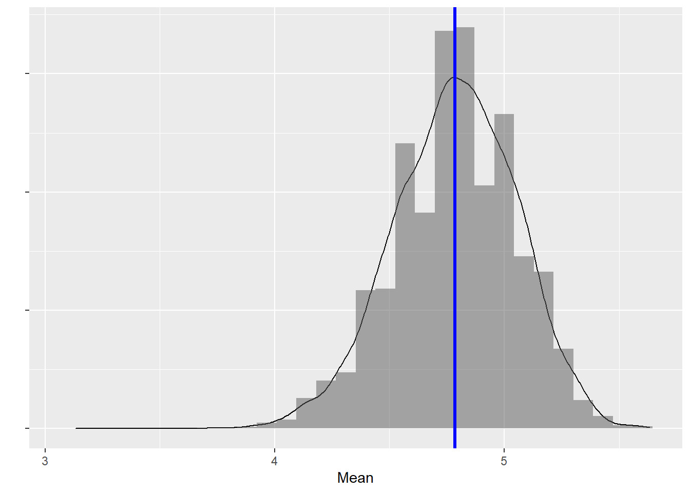
But what happens when we take samples from this set of 1000 throws?
sampleMeans <- c()

# I'm going to take ten thousand samples of size 30, and plot the means from them
for (i in 1:10000) {
    sampleMeans[i] <- mean(sample(biasedData$result, 30, replace = TRUE))
}

samplingDist <- ggplot() +
                  aes(sampleMeans) +
                  geom_density(aes(y = ..density..)) +
                  geom_histogram(aes(y=..density..), alpha = 0.5) +
                  geom_vline(xintercept = mean(sampleMeans),col="blue",lwd=1.1) +
                  ylab("") +
                  xlab("Mean") +
                  theme(axis.text.y = element_blank())

samplingDist
The sample means are distributed symmetrically around the mean! This seems to be true regardless of the underlying distribution the samples were taken from.
Concluding thoughts
I’m not going to go any deeper into the technical aspects of the law of large numbers and the central limit theorem. This post is intended to serve as a friendly introduction to the world of statistics and research. Later posts may go deeper into the specifics that have been mentioned or alluded to within this post regarding the central limit theorem etc. But the take home message is this: If we can take sample measurements from a distribution that we know follow specific rules if we fulfill certain criteria regarding sample size etc. then we can construct models based on that data to simulate reality. For instance I can conclude based on my data that the biased die is indeed biased (how I would go about that is the subject of a different post). We have seen how the gambler’s fallacy can make sense in that small samples are expected to be heavily skewed one way or another every now and then, and that is OK, but on average expected probabilities prevail.